The Dyson-Wyld equations

In the diagrammatic series for the Green's function one may perform the partial Dyson's summation over one-particle irreducible diagrams. This results in the Dyson equation for the Green's functions:

$$G({\bf k},\omega) = \frac{1}{\omega-\omega_0(k) +i0 -\Sigma({\bf k},\omega)}$$ (68)

where the ``mass operator'' $\Sigma ({\bf k},\omega )$ gives the nonlinear correction to the complex frequency $\omega_0({\bf k})+i 0$ due to the interaction (2.19). This is an infinite series with respect to the bare amplitude $V({\bf k},{\bf q},{\bf p})$ (2.20), dressed Green's function (4.2) and double correlation function $n({\bf k},\omega)$ (4.3). All of the contributions of the second and fourth order in $V$ are shown on Fig 1(b).

We have not specified the direction of arrows on Fig 1(b); each diagram should be interpreted as a sum of diagrams with all possible directions of arrows compatible with vortex $V({\bf k},{\bf q},{\bf p})$, describing the three-wave processes $1\leftrightarrow 2$. For example, diagram (a) on Fig 1(b) corresponds to three diagrams shown on Fig 2. The diagram (a4) on Fig 2 describes the nonresonant process $0\leftrightarrow3$ which is not essential for our consideration.

With the help of the similar Dyson's summing of one-particle irreducible diagrams, one can derive Wyld's equation for $n({\bf k},\omega)$:

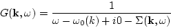
$$n({\bf k},\omega) = \vert G({\bf k},\omega)\vert^2\left[D({\bf k},\omega )+\Phi({\bf k},\omega)\right] \ .$$ (69)

Here $D({\bf k},\omega)$ is the correlation function of white noise,

$$(2\pi)^4 D({\bf k},\omega)\delta({\bf k}-{\bf k}')\delta(\omega-\omega') = \left<f({k \omega}) f^*({k'\omega'})\right>,$$ (70)

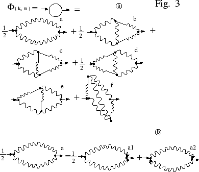
and the mass operator $\Phi ({\bf k},\omega )$ describes the nonlinear corrections to $D({\bf k},\omega)$. This is an infinite series with respect to the same objects $G({\bf k},\omega)$, $n({\bf k},\omega)$ and $V({\bf k},{\bf q},{\bf p})$. All diagrams of the second and fourth order are shown on Fig 3(a).

We also have not specified arrow directions in the diagrams for $\Sigma ({\bf k},\omega )$ and $\Phi ({\bf k},\omega )$. In complete analogy with diagrams for $G({\bf k},\omega)$ one diagram on Fig 3a corresponds to two diagrams (a1) and (a2) on Fig 3b. All the rest diagrams for $\Phi ({\bf k},\omega )$ reproduces in the same way - one chooses all possible directions of arrows and discards those which incompatible with definition of vertex $V$ (see Fig 1a).

Figure 3: First terms in the diadrammatic pertubation expansion for mass operator $\Psi{({\bf k},\omega )}$.