Objects of Diagrammatic Technique

Let us define the ``bare'' Green's function of Eq. (2.24) as

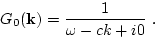$$G_0({\bf k})=\frac{1}{\omega-c k+i 0}\ .$$ (63)

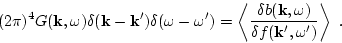
One may see from (2.24) that this function describes the response of the system of noninteracting acoustic waves on some external force. We added in the denominator the term $+i 0$ by requirement of causality. We remark that causality (the arrow of time) is introduces in the perturbation approach by the limit $t\to\infty$ and the fact that ${\rm sgn}t$ appears in (1.7). Next we introduce the ``dressed'' Green-function which is the response of interacting wave systems on this force:

$$(2\pi)^4 G({\bf k},\omega)\delta({\bf k}-{\bf k}')\delta(\om... ...elta b({\bf k},\omega)} {\delta f({\bf k}',\omega')}\right>\ .$$ (64)

We will be interested also in the double correlation function $n({\bf k},\omega)$ of the acoustic field $b,\ b^*$

$$(2\pi)^4 n({\bf k},\omega)\delta({\bf k}-{\bf k}')\delta(\om... ...ga') =\left<b({\bf k},\omega)b^*({\bf k}',\omega')\right> \ .$$ (65)

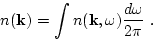
The simultaneous double correlator of the acoustic field $n({\bf k})$ is determined by

$$(2\pi)^3 n({\bf k}) \delta({\bf k}-{\bf k}')= \left<b({\bf k},t)b^*({\bf k}\lq ,t)\right>\ .$$ (66)

This is related to the different-time correlators in the $\omega$ representation $n({\bf k},\omega)$ as follows:

$$n({\bf k})=\int n({\bf k},\omega) \frac{d \omega}{2\pi}\ .$$ (67)

The Green's and correlation functions together with the bare vertex $V({\bf k},{\bf q},{\bf p})$ (2.20) are the basic objects of diagrammatic perturbation approach which we are going to use (see Fig 1a).

Figure 1: Panel (a): Basic objects of diagrammatic pertubation approach. Panel (b): First terms in the expansion of mass operator $\Sigma{({\bf k},\omega )}$.

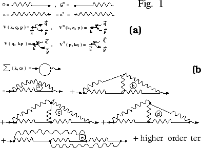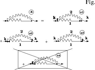
Figure 2: Diagrams (a) from Fig.1 with specified directions of arrows.