Equations of Motion and Canonical Variables

Consider again the Euler equations for a compressible fluid (2.1). The enthalpy of a unit mass $w=E+p V$ is equal to the derivative of internal energy of unit volume $\varepsilon(\rho)=E\rho$ with respect to fluid density: $w={\delta\varepsilon/\delta\rho}\$. As a result of direct differentiation with respect to time, it is readily evident that equations (2.1) conserve the energy of the fluid

$${\cal H}=\int[\rho v^2/2+ \varepsilon(\rho)]\,d{\bf r}\ .$$ (33)

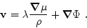
One can show (and see for example[1]) that Eqs. (2.1) may be written in the Hamiltonian form:

$$\partial\rho/\partial t = \delta{\cal H}/\delta\Phi\;,\quad \partial\Phi/\partial t=-\delta{\cal H}/\delta\rho\;,$$ (34)

$$\partial\lambda/\partial t = \delta{\cal H}/\delta\mu\;, \quad \partial\mu/\partial t=-\delta{\cal H}/\delta\lambda\;,$$ (35)

if the velocity ${\bf v }({\bf r}, t)$ is presented in terms of two pairs of Clebsch variables $(\rho,\Phi)$ and $(\lambda ,\nu)$ as follows,

$${\bf v}=\lambda{{\bbox\nabla}\mu\over\rho}+{\bbox\nabla}\Phi\ .$$ (36)

Here the energy (2.11) is expressed in terms $(\rho,\Phi)$ and $(\lambda ,\nu)$ so that (2.14) becomes the Hamiltonian of the system. As seen from (2.14), the case with $\lambda=0$ or $\mu=$const corresponds to potential fluid motions which are defined by a pair of variables ($\rho,\Phi$) according to equations (2.12). It is convenient to transform in the $\bf k$-representation from the real canonical variables, $\Phi({\bf k}),\rho({\bf k})$ to the complex ones $b({\bf k})$ and $\ b^*({\bf k})$,

$$\Phi({\bf k}) = -i\sqrt{(c /2\rho_0k)} [b({\bf k})-b^*(-{\bf k})]\,,$$ (37)

$$\delta\rho({\bf k}) = \sqrt{(\rho_0 k /2\c)}[b({\bf k})+b^*(-{\bf k})]\ .$$ (38)

Here $\delta\rho({\bf k})=[\rho({\bf k})-\rho_0({\bf k})]$ is the Fourier transform of density deviation from the steady state.